Resolving very complicated science and engineering problems

- Download Aviation project source code - 1.86 MB
- Download Aviation + Control Systems project source code - 2.03 MB
- Download Category Theory project source code - 983.44 KB
- Download Astronomy Express project source code - 2.52 MB
- Download Imported Trajectory project source code - 131.58 KB
- Download Dynamical Atmosphere project source code - 196.94 KB
- Download Gravity project source code - 185.89 KB
- Download Aggregate Library project source code - 855.44 KB
- Download Asrtoframe project user guide - 1.94 MB
- Download Category Theory project user guide - 467.03 KB
- Download installer of Hipparcos and Tycho catalogue of stars - 121.6 KB;
- Dowlload automation equipped working place source code - 770.03 KB
Other useful resources:
1. Introduction
I have found that I can easy resolve very complicated science and engineering problems using my software. But it is very difficult to teach others. I am trying different methods of teaching. One of them is "live parallel" with well known software. Here I describe live parallel with The Incredible Machine. I do not need dithyrambs. I am looking for readers which have strong interest to my ideas. My ideas are not fast-food. My articles are also my excercises explanation of my ideas. And feedback of readers is are very helpful. So I am writing this article in real time mode
2. Background
I find that The Incredible Machine very useful game. When I was a child I did not have computer. But I had constructed Grandiose Projects in my mind. These projects were very close to The Incredible Machine tasks. These tasks were not realistic. Then I had learned math, physics and could solve realistic tasks. My software is realistic. But I also is being use unrealistic samples for teaching. Although The Incredible Machine is not realistic it is very useful for education. Here I will compare my software with The Incredible Machine.
3. Common features of Framework and The Incredible Machine
3.1 Qualitative variety of phenomena
The Incredible Machine contains a large qualitative variety of phenomena. It includes geometry, mechanics, electricity, pneumatic, explosions and even psychology of animals. A lot of advanced engineering software do not contains such variety. For example LabVIEW contains a lot of components, but LabVIEW do not have mechanical components. Similarly the Framework has mechanics, electricity et cetera.
3.2 Interaction of phenomena
The Incredible Machine has interaction of phenomena. For example, if a ball is close to fan than air flow acts on the ball. Typical Framework example is an action of Earth's magnetic field on spacecraft motion.
3.3 Declarative approach
For simulation of air flow action on ball we need set ball position only. We do not need following imperative: "Flow, act on the ball". Action is provided implicitly. The same words we can say about action of Earth's magnetic field on spacecraft motion.
3.4 Relation to Grandiose Projects
Grandiose Project has a lot of qualitatively different phenomena. For example if electrical device is near heat source then electrical processes depend of heat. So there is interaction between phenomena. Declarative approach makes software development robust and easy.
4. Difference between Framework and The Incredible Machine
The incredible machine devoted to unrealistic phenomena only. The Framework is used for complicated science and engineering problems.
5. Getting Started
This article will become really interesting when I will fulfill it by samples. I am writing it mostly at weekends. And first sample will appear in next weekend. One objective of this article is research of popularity. This article does not contain any code yet. But current number of visits is my own record. I think that such popularity caused by article name. But I strictly comply following CodeProject rule: "Article should contain code". I think this rule do not contradicts my research. Moreover other members of CodeProject can enlarge their popularity by usage of good article name. I find that it is not interesting write article about soft that was developed later, since the Framework can resolve unpredictable tasks. So I will be thankful to reader who asks me to resolve unpredictable task. It would be a good test for the Framework. Maybe I will include some of suggested tasks into this article. If one of readers would construct a sample of incredible machine then it would be excellent. I shall include this sample into this article. I had constructed incredible machines many years and do not have very interest for this occupation. I would like that another developers be able construct incredible machines.
5.1 Kinematics
5.1.1 Very simple sample
This sample is "Hello world" of the Framework. It is presented in following picture:
We have a point Motion which is moving relatively point Base. We can simulate this picture by the Framework:
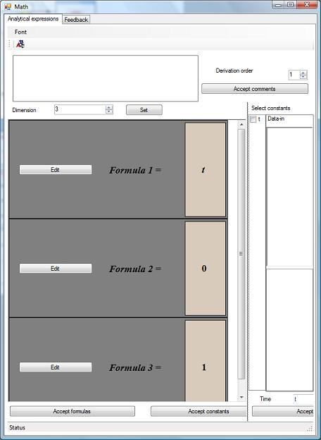
Derivation order is equal to 1 for calculation of relative velocity.
The Math object is used by Motion object. Properties of Motion object are presented below:
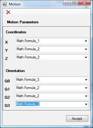
This means that x - coordinate of Motion object is defined by Formula 1. Other coordinates and Q1, Q2, Q3 components of orientation quaternion are defined by Formula 2. The Q0 component is defined by Formula 3. Since Formula 1 = t, Formula 2 = 0 and Formula 3 = 1 we have following 6D motion law:
x(t) = t;
y(t) = 0;
z(t) = 0;
Q0(t) = 1;
Q1(t) = 0;
Q2(t) = 0;
Q3(t) = 0;
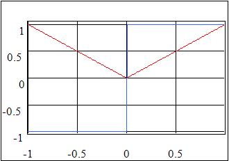
The Measurements object measures parameters of Motion object motion relatively the Base object. The Graph object indicates parameters of relative motion:
5.1.2 Sample with medium frame
Kinematic picture of this sample is presented below:
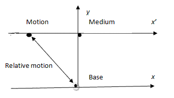
We have three frames. The frames are named as Base, Medium and Motion. The framework shows this picture by the following way:
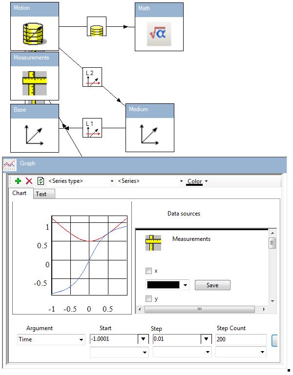
The L 1 and L 2 are geometric links. The L 1 links means that motion of Medium frame is considered relatively to Base frame. Similarly link L 2 means that motion of Motion frame is considered relatively Medium frame.
The Medium frame has following properties:
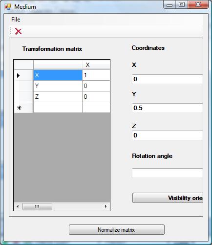
These properties mean that relative coordinates of Medium frame are equal to:
x = 0;
y = 0.5;
z = 0;
Properties of Motion are the same as in chapter 5.1.1. Arrows between Measurements - Base and Motion - Measurements mean that Measurements provides parameters or Motion frame motion with respect to Base. The Chart object indicates relative motion parameters:
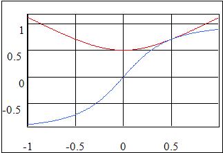
Red curve is relative distance and blue one is relative velocity. Note that differentiation of distance is implemented implicitly. We only put frames and automatically obtained distance derivation. The Framework performs symbolic differentiation. But differentiation is performed implicitly. Formulas do not contain functions which are presented in above charts. These charts are defined by relative positions of frames. But engineer have a lot of other problems which are outside calculation of explicit dependencies.
5.1.2 Sample with rotated frame
Readers. Excuse me please during construction of next sample I has found a bug. The bag is fixed. If you have already downloaded Aviation project you should download it once again. The Framework is being continuously developed. Previous samples have been tested.
Kinematics of this sample is presented below: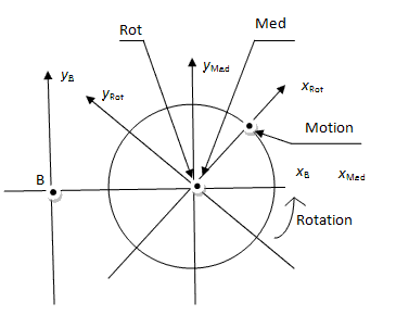
This sample contains four frames. Properties of their coordinat systems are presented below:
| Frame | Frame center | Coordinates |
| Base | B | xB,yB |
| Medium | Med | xMed,yMed |
| Rotated | Rot | xRot,yRot |
| Motion | Mot | xMot,yMot |
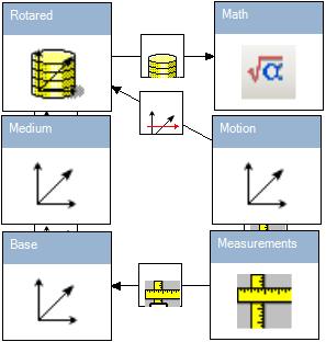
Base - Medium - Rot - Motion
The linkMedium - Rot
is not rigid. Its motion low is presented below:x(t) = 0;
y(t) = 0;
z(t) = 0;
Q0(t) = cos(at);
Q1(t) = 0;
Q2(t) = 0;
Q3(t) = sin(at);
where t is time and a is constant.
It means that Rot is rotated with respect to Medium. Angular velocity is constant.
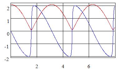
Following chart presents relative motion of Motion frame with respect to Base frame:
Writing temp of this article is very slow. But my experience tell me that understanding of my ideas is more slow. Readers which have strong interest to my ideas can download above samples and try to develop other. I will accept any questions and suggestions.
Wait next weekend.
5.1.3 A complicated set of frames
Set of frames can be more complicated. Complicated set of frame is presented below:
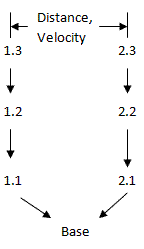
The framework diagram which correspond to this set of frames is presented below:
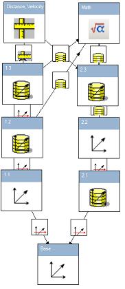
Now we can calculate relative distance and velocity between frame 1.3 and 2.3. We have following complicated curves:
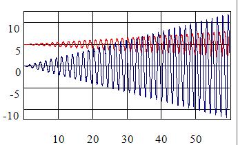
This sample can be regarded as too artificial. But I know a lot of engineering problems with similar configuration. Reader can find these samples in my articles Virtual Reality at Once and "Control systems. Processing of signals"
5.1.4 Trajectory import
Today (02/07/2008) I have received a message about lack of code. Thanks. Indeed this article is not interesting without code samples. So I have prepared a little code for this article. You can download it:
This code is used in framework for kinematics. Third party software is used by IObjectFactory interface. Sample code contains class
ComplicatedTrajectorythat implements this interface:
/// <summary>
/// Names of objects
/// </summary>
string[] IObjectFactory.Names
{
    get { return new string[] {"Complicated Trajectory"}; }
}
/// <summary>
/// Gets object by name
/// </summary>
/// <param name="name">Name of object</param>
/// <returns>The object</returns>
ICategoryObject IObjectFactory.this[string name]
{
    get { return new ComplicatedTrajectory(); }
}
The Names property contains names of exported objects. Property this returns object by name. Class ComplicatedTrajectory impelements IObjectTransformer interface:
 /// <summary>
/// Calculates trajectory parameters
/// </summary>
/// <param name="input">Input parameters</param>
/// <param name="output">Output parametres</param>
void IObjectTransformer.Calculate(object[] input, object[] output)
{
    // Input extraction
    double a = (double)input[0];
    double b = (double)input[1];
    double t = (double)input[2];
    // Calculation
    double x = a * t;
    double y = x * t;
    double z = y * t;
    double phi = Math.Atan(b * t);
    double Q0 = Math.Cos(phi / 2);
    double Q1 = 0;
    double Q2 = 0;
    double Q3 = Math.Sin(phi / 2);
    // Output filling
    output[0] = x;
    output[1] = y;
    output[2] = z;
    output[3] = Q0;
    output[4] = Q1;
    output[5] = Q2;
    output[6] = Q3;
}
This code calculates parameters of trajectory. The t is time, a and b are constants. Meaning of output parameters is evident. So we have third party project and we would like use it for kinematics. Following picture demonstrates this usage:
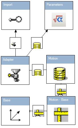
The Import is imported object. It has following properties:
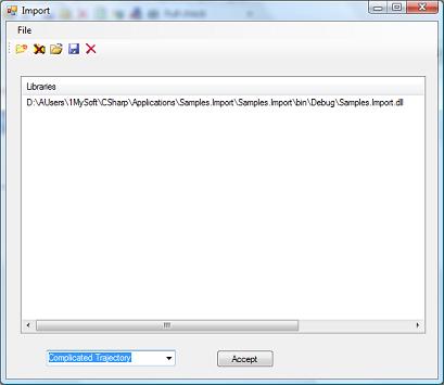
One of properties is *.dll filename. Second one is object name. Note that *.dll is saved in file *.cfa and then project does not depend on initial *.dll file existence. Full diagram enable us to define Motion object trajectory. The Motion - Base object performs relative motion measurements:

Red, blue and green curves a relative x, y and z coordinates respectively. Note that we cannot define velocities since imported library do not contain derivations. User shoud implement a set of interfaces for definition of velocities.
5.2 Dynamics
Realistic mechanics requires differential equations of dynamics. The framework has differential equatioins' component. This component can be used for mechanics. Here we consider a set of samples.
5.2.1 Mechanical oscillator
This sample is classical. It is presented below:
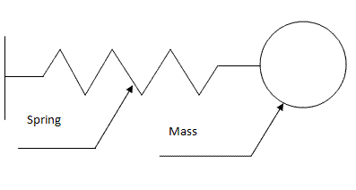
This sample is described by following differential equations:
dx/dt = v;
dv/dt = -av - bx;
where x is coordinate and v is velocity. The "-bv" is caused by damping factor and "-bx" is caused by force of string. The framework picture is presented below:
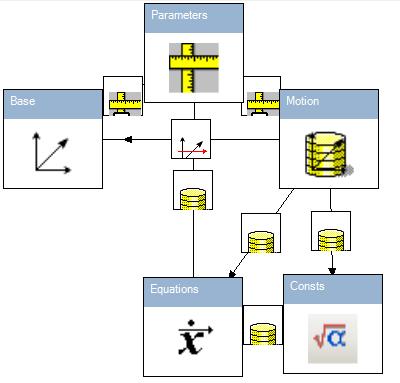
Here the Equations object contains dynamical differential equations. Chart of relative distance and velocity is presented below:
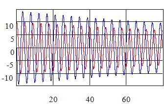
We have damping oscillations as it have been expected.
5.2.2 Jump
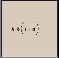
The incredible machine contains jumps. Adequate realistic description of jumps provides Dirac delta function. The framework has it. Framework sample of oscillations with jump is presented below:
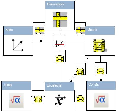
The Jump object contains Dirac delta function:
So we have jump at following charts:
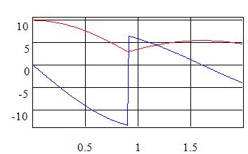
At this chart red curve is a distance and blue curve is a velocity. The distance is a continuous function. But its derivation (distance) has a point of discontinuity (Jump) as it has been expected.
5.2.3 Realistic Sample. Earth artificial satellite
Hello everybody. I have updated source code of Aviation project ad uploaded it. Let us consider realistic sample. Earth artificial satellite had already been considered in article 6 and atricle 12. Here I would like to compare imperative approach with declarative one. This sample requires import of third party software (external libraries). The Asrtoframe project user guide (1.94 MB) contains import instruction. Also reader can download source code of third patry software:
The task is presented in following picture:

We have a Satellite and would like simulate its motion parameters with respect to Ground Frame.
5.2.3.1 Imperative approach
Imperative picture is presented below:
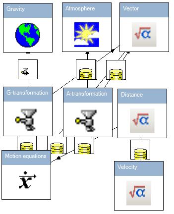
The Gravity and Atmosphere are imported objects. These objects are used in Motion equations object which contains ordinary differential equations of satellite. The Distance and Velocity objects contain explicit formulas of relative distance and velocity:
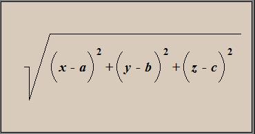

The a, b and c are coordinates of Ground Frame. These coordinates are constants which belong to Distance object. Values of constants you can find in Distance properties:
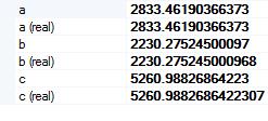
Result of simulation is presented in following charts:
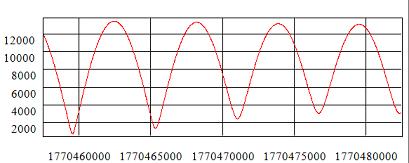
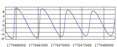
These charts show relative distance and relative velocity respectively.
5.2.3.2 Declarative approach
The picture of declarative approach is presented below:
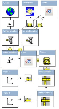
This picture do not contain explicit formula of distance. Instead we have reference frames. The Motion frame is reference frame of satellite. This frame uses parameters Motion equations object. The Frame 1 is ground frame. Its coordinates are presented below:
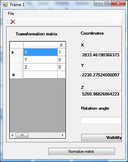
This coordinates are equal to coordinates of Ground Frame in imperative approach. We also have Frame 2. This frame is presented for demonstration of advantages of declarative approach. Objects Measurements 1 and Measurements 2 perform relative measurements "Motion - Frame 1" and "Motion - Frame 2" respectively. Simulation result is presented in following charts:


Every chart contains two curves which correspond to Frame 1 and Frame 2 respectively. Coordinates of Frame 1 are equal Ground Frame coordinates to imperative approach coordinates. So one curve on each chart is the same as in imperative approach.
5.2.4 Mechanics and differentiability. Declarative approach once again
Differentiability has important role in mechanics. However engineer should not be too overloaded by differentiability issue. A lot of work should be performed declaratively. Let us consider following mechanical task. We have a moved object and its coordinates are time functions x(t), y(t), z(t). If we would like to install (virtual) inertial navigation system on this object then these functions should be twice differentiable. However second derivations can be discontinous. If these functions are not twice differentiable then attempt of inertial navigation system installation results to exception. Twice differentiable function can be obtained by natural way. For example they can be obtained from following dynamics equations:

In these equations Fx, Fy, Fz can be discontinous. But Vx , Vy, Vz are continuos with discontinous derivations. Functions x(t), y(t), z(t) are twice differentiable with discontinous second derivations. Let us consider how framework operates with differentiability. Suppose that we would like to solve following system of differential equations:
![]()
Here a(t) is discontinous function:

Solution of this problem by framework is presented below:

Here Input component contains above discontinous function. The Diff Equations components is solver of above differential equation system:

Now we would like consider x as twice differetiable function. We can do it by defining following properties of variables:

Here x is twice differentiable and y is once differentiable. If we try increase order of derivavative of every variable then exception will be thrown since x is twice differentiable and y is once differentiable only. The Diff Test component performs test of this sample by (twice) differentiation of x:

If we try to define third derivation of x, then exception will be thrown.
Test result is presented in following picture:

Red curve is x(t), green and blue curves are its first and second devivations respectively.
5.3 Physical fields
Physical fields are implemented abstractly. It enables us use them in radiophysics, magnetism, pneumatics. Moreover physical fields provides advantages of declarative approach. Development becomes more laconic. Let us consider some examples.
5.3.1 Pneumatic
Let us consider a "Fan and Ball" sample:

We have Base reference frame. The Y and Z are its axes of reference. Axis X is perpendicular to Y and Z. The picture shows wind rose of fan. We would like simulate pneumatics as physical field. So we have constructed following diagram:

This picture has three parts: Fan, Ball and Bridge. Fan is a source of physical field. Ball is a consumer of field. The Bridge performs interoperability. We have field interoperability and kinematic interoperability. Let us consider all subjects of this picture.
5.3.1.1 The Fan
Fan has a reference frame (Field Frame) and physical field (3D Field). The field is strongly linked with frame:


Double and Double[3] respectively. So kx is scalar - vector product. It this formula is used by 3D Field. The x is relative vector and k is wind rose coefficient defined by formula 
where![]() phi is angle between reference line and z - axis of Fan.
phi is angle between reference line and z - axis of Fan.
r is a distance between field source (Fan) and sensor
.
5.3.1.2 Bridge
Bridge contains common Base reference frame and declarative link Field between 3D Field (of Ball) and Sensor. This link means that Sensor is a sensor of 3D Field. Any field can have a set of sensors which have different positions and orientations.
5.3.1.3 The Ball
Configuration of the Ball is presented below:

The ball has reference frame (Ball) and a sensor (Sensor). Ball and Sensor are rigidly linked. Sensor is a sensor of Fan pneumatic field. Output of Sensor is used (through Disass) in differential equations Equation. Otherwise Equation result is used for the reference frame Ball motion simulation.
5.3.1.4 Declarative approach
Declarative approach enables us simulate a lot of properties by changing of few parameters. For example we can change orientation of Field Frame (frame of Fan). In result the Ball trajectory will be changed. Two different Field Frame orientations are presented below:


These orientations are defined by transformation matrix. Change of orientation results to following change of the Ball trajectory. You can compare two charts below:


These charts shows time evolution of z - coordinate of the Ball. However the Fan position and orientation do not force only the Ball trajectory. Relative position of Ball with respect Fan depends on position of Fan.
5.3.2 Dipole radiation + Kinematics
Here we use kinematics picture which is considered in 4.1.2. Besides kinematics we will consider dipole radiation. Full picture is presented below:

We have three parts: Dipole, Bridge and Receiver. Let us describe them.
5.3.2.1 Dipole
Dipole uses kinematics which is used in 4.1.2. The Field Calculation object contains calculation of dipole field parameters: amplitude and phase. Amplitude formula is presented below:

Here m is dipole moment, r is distance, x is relative radius vector. The cross product means vector cross product. In fact this formula coincides with one dipole radiation formulas.
The Field object contains two components:

These components are Field Calculation.Formula_1 and Field Calculation.Formula_2. First one is vector and second one is scalar. First component physically means amplitude. Second one means phase.
5.3.2.2 Bridge
Bridge contains the Base object and the Link link. The Base is common reference frame. The Link is declarative link between source of field and receiver.
5.3.2.3 Receiver
Receiver contains Sensor of field and Receiver object. The Receiver object performs processing of Sensor information by following expression:

Here x, y, z are components of Field amplitude, o is angular frequency, t is time and p is phase. Note that this formula is rather reasonable interpretation than realistic receiver formula.
In result we have following receiver signal:

Let us provide its qualitative explanation. First of all we have amplitude peak. Also we have monotone decrease of frequency. These phenomena can be explained by motion. Motion chart is presented below:

Red curve is distance between field source and receiver. Blue curve is relative velocity. Amplitude peak is caused by distance extremum. Monotone decrease of frequency is caused by monotone increase of relative velocity.
5.3.3 Dipole radiation + Kinematics + Envelope detector
Let us add to previous situation envelope detector. The envelope detector can be implemented by following circuit:

This circuit is simulated by the following way:

The Rectifier object contains formula of rectifier. The Filter object simulate dynamic object with following transfer function:

where  .
.
The Filter object is in fact a low-pass filter with following frequency response:

Following chart shows result of envelope detector:

Red curve is output of Rectifier. Blue curve is output of Filter. So blue curve is in fact envelope (with coeffcient). Reader need Aviation + Control Systems project for this sample:
5.3.4 Dipole radiation + Kinematics + Frequency detector
Frequency dectector can be implemeted by usage of high-pass filter. Scheme of filter is presented below:
Filter has following transfer function: . Frequency response and phase response of the filter are presented below:

Following scheme is used for amplitude variation compensation:

This scheme contains envelope detector (see 5.3.3). Result of scheme bottom branch is divided by output of envelope detector.
The framework picture of frequency detector is presented below:

Left part contains envelope detector (see 5.3.4). Right part contains high-pass filter (Diff) rectifier (Rectifier 1) ald low-pass filter (Filter 1). The Detector object divides output of Filter 1 by output of Filter. Output of Detector is proportional to frequency. It is presented below:

Such behavoir of frequency can be easy explained by following chart of relative velocity:

Reader need Aviation + Control Systems project for this sample:
5.3.4 Dipole radiation + Kinematics + Phase detector
Here we consider application of phase detector. Situation is presened in following picture:

Dipole radiator (Dipole) is moved. We have two receivers 1 and 2. Distances D1 and D2 are different. The d parameter is called base. So we have phase difference. Here we will define this difference by correlation method. This method can be expessed by following formulas:

where Ixx , Iyy , Ixy are correlation integrals which can be calculated by the following way:

where x(t) and y(t) are singnals of recievers.
Calculation is divided on two steps. First step is simulation and recording of signals. Second step contains calculation by correlation method.
5.3.4.1 Simulation and recording
Configuratiton of this step is very similar to configurations whis was considered in 5.3.2 and 5.3.3. But here we have two receivers istead one. Fragment of the situation is presented below:

Every receiver has own reference frame (Frame 1 and Frame 2). We can change parameter d by changing coordinates of these frames. Simulation gives following signals of receivers:

Red curve is signal of Receiver 1, blue curve is signal of Receiver 2. Now we can record these signals and go to next step.
5.3.4.2 Calculation by correlation method
Calculation scheme is presented below:

Left part squares contain recorded signals. Red/Blue curve is signal of first/second receiver. Recursive element calulates necessary integals. Right object calulates cosine of phase difference. In result we have following chart of the cosine:

It is clear that this chart corresponds to considered kinematics. If we multiply d (base) by 2 then we will obtain following chart of phase cosine:

This result is evident.
5.4 Regression
Nonlinear regression in statistics is the problem of fitting a model:
![]()
to multidimensional x,y data, where f is a nonlinear function of x, with regression parameter θ. I find that pure regression software is not quite effective. It should be integrated into more common framework. I had been considered application of regression to determination of orbits of artificial satellites problem. The standalone regression soft could not resolve such problems. I had considered regression in article 2. Here I will consider new essential feature. It is F-distribution. Why F-distribution? We need it for looking for appropriate math model. Statisics knows that more complicated model is not more adequate. For example if secection contains 20 points then usage of 19 - degeree polynom leads to zero residue. So we can think that 19 - degree polynom is ideal model. But in fact this polynom reflects rather errors than real physical picture. Here we will consider following sample:

Top part of this picture contains selection. Left part contains 4-degree polynomial model, right part contains 5-degree one. The residuals of 5-degree model is less than 4-degree one. It is presented in following picture:

Blue curve is 4-degree polynomial approximation and red curve is 5-degree polynomial approximation. The 0.383037446029811 of Fisher is significance level of F-distribution statistical criteria. Roughly speaking this number is chance that 5-degree polynom is better than 4-degree one. Usually statistics prefer the 4-degeree polynom in this case.
5.5 Algebraic topology
At the beginnig of XX century General relativity and Quantum mechanics had being factastic ideas reather reality. But these brunches of science are everyday engineering tools now. Present day theoretical physics operates with XX and XXI centuries math. This math includes algebraic topology. Scientist and futurist Dr. Michio Kaku told about making what was once considered impossible technology into reality. I had begun implement this idea. Category Theory project is devoted to this purpose. I know a lot of cases when General Relativity and Classical Mechanics had been used in the single project. So I think that kinematics, dynamics, field theory and algebraic topology should have universal software framework. Framework should be common for all branches of science. Algebraic topology could not be undrestood at once. This chapter is rather inspiration. Reader need Category Theory project and its user guide:
- Download Category Theory project source code - 983.44 KB
- Download Category Theory project user guide - 467.03 KB
Here I would lilke define some invariants of space X which is direct product of real projective space and Klein bottle ![]() . Later I will denote projective space by R. Anatoliy Fomenko expressed these spaces by following way:
. Later I will denote projective space by R. Anatoliy Fomenko expressed these spaces by following way:

5.5.1 Calculation of homology
Homology can be calculated by chain complexes. These complexes are presented below:
![]()
Chain complexes of projective space and Klein bottle are well known. We would like calculate it for direct product. Chain complex of Klein bottle is presented below:

Framework represents this chain complex by following way:

Chain complex of projective space is presented below:
![]()
Properties of objects and arrows of this diagram can be edited by right mouse click on squares. So let us calculate homology groups of X. First of all we will construct chain complexes of projective space and Klein bottle:

Top complex is complex of Klein bottle. Bottom complex is complex of projective space. Gray squares K and R are complexes as single objects. Chain complex of X is tensor product of these complexes. We can construct it (see user guide).
Now we have chain complex of X:

Now we can calculate homology of X (see user guide):

Top complex is chain complex of X. Bottom row of squares are homology groups of X.
5.5.2 Homology with coefficients in Z/2Z
Homology with coefficients can be calculated by application of tensor product functor ![]() . Calculation scheme is prezented below:
. Calculation scheme is prezented below:

Top complex is chain complex of X. Bootom part contains complex of X as single object and tensor product functor. We perform tensor product functor ![]() .
.
5.5.3 Calculation of cohomology
Cohomology can be calculated by application of Hom(Z,-) contravariant functor. Framework presents this functor by following way:

Left square represensts Z group. Right square represents functor. Arrow between squares means association. Application of this functor provides cochain complex. Cohomolgy are homology of this cochain complex. User can download full calculation of cohomolgy of X below:
6. Advanced Sample. Controlled spacecraft
A spacecraft is a very good example of the incredible machine. It has a lot of systems and aggregates. The picture belows presents Mir orbital station:
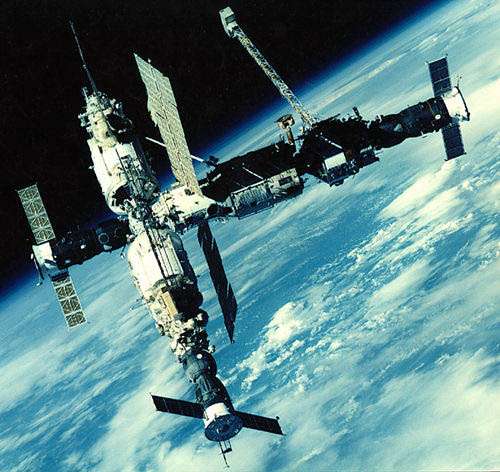
This station is a subject of History. But building blocks of the framework enable us construct new spacecrafts and orbital stations. The station is a very complicated mechanical object. It is not rigid body. It has solar cell panels. These panels are elastic. The station is stabilizied by gyros. Moreover station configuration is not constant. I had already considered mechanical aspects in article 9. This chapter contains interoperability of mechanics and other phenomena.
6.1 Mechanics
We will use aggregate designer for mechanics simulation. Why aggregate designer? Indeed mechanical equations are well known long time ago. But software development for simulation of complicated mechanical objects is not quite easy task. Aggregate designer make this task much easier. Aggregate designer is integrated into framework. This fact enables us provide interoperability of mechanics with physical fields. So it is easy to simulate action of magnetic fields on mechanical objects. I will consider this task below. Now we would like to create mechanical model of spacecraft from models of its modules. Typical spacecraft module is schematically presented below:

This module has own coordinat system OXYZ. Also it has places of connections. We can connect other modules to this module. Behavior of module is defined by following kinematic parameters:
- Radius vector r;
- Velocity V;
- Orientation quaternion Q;
- Angular velocity
 .
.
But module is not rigid in general. And these parameters are not parameters of module. These parameters are rather parameters of one point of module. In this article we suppose that these parametres are parameters of origin of OXYX coordinat system. Since module is not rigid it has additional degress of freedom. These degrees of freedom can be interpreted as generalized coordinates qi (i= 1,...,n). Instant state of module is defined by following parameters:
![]()
I will call them state variables. Parameters:
![]()
will be called accelerations. Mechanical equations define accelerations by state parameters. Accelerations near connecton can be defined by following way:

where i is number of connection. Other variables are matrixes which depend on state variables. Let us connect two modules:

Both modules have equal acceleration near connection. First module acts to second one by force F12 and mechanical momenum M12. Similarly second module actcs to first one by force F21 and mechanical momenum M21. Following equations:
F12=-F21;
M12=-M21;
are well known. Mechanical equations of module can be represented by the following way:

In these expessions accelerations are independent variables. Fi (Mi) is force (mechanical momentum) of i- h connected module. Other vector and matrix parameters denend on state variables. Adding following evident expressions:

results to linear by accelerations system of equations. This system enables us to find all acceleratios. So we have mechanical equations. It is worth to note that this system is redundant. If n1(n2) is number of freedom degrees of first (second) module then system has n1+n2 degrees of freedom. However aggegate has n1+n2-6 degrees of freedom. The framework can avoid this redundancy. But I will not describe it in this arctile.
There are a lot of module types. Prorammatically all of them implement following interface:
/// <summary> /// Aggregable Mechanical Object /// </summary> public interface IAggregableMechanicalObject { /// <summary> /// Number of degrees of freedom /// </summary> int Dimension { get; }/// <summary>
/// Number of connections /// </summary> int NumberOfConnections { get; }
/// <summary>
/// State of object /// </summary> double[] State { get; }
/// <summary>
/// Internal acceleration /// </summary> double[] InternalAcceleration { get; }
/// <summary>
/// State of connection /// x[0] - position, x[1] - quaternion, /// x[2] - linear velocity, x[3] - angular velocity /// </summary> /// <param name="numOfConnection">Number of connection</param> /// <returns>State of connection</returns> double[] this[int numOfConnection] { get; set; }
/// <summary>
/// Calculates transformation matrix from genrealized coordinates to /// acceleration of connection /// </summary> /// <param name="numOfConnection">Number of connection</param> /// <returns>The transformation matrix</returns> double[,] GetAccelerationMatrix(int numOfConnection);
/// <summary>
/// Gets matrix of forces /// </summary> /// <param name="numOfConnection">Number of connection</param> /// <returns>The matrix of forces</returns> double[,] GetForcesMatrix(int numOfConnection);
/// <summary>
/// Gets internal acceleration /// </summary> /// <param name="numOfConnection">Number of connection</param> /// <returns>Internal accceleration</returns> double[] GetInternalAcceleration(int numOfConnection);
/// <summary>
/// Gets connection force /// <summary> /// <param name="numOfConnection">Number of connection</param> /// <returns>Connection force</returns> double[] GetConnectionForce(int numOfConnection);
/// <summary>
/// Children objects /// </summary> Dictionary<IAggregableMechanicalObject, int[]> Children { get; }
/// <summary>
/// The is constant sign /// </summary> bool IsConstant { get; }
/// <summary>
/// Parent object /// </summary> IAggregableMechanicalObject Parent { get; set; }
}
I will consider samples of modules below. Here I describe this interface. Meaning of this interface members is presented in following table:
| Number | Member | Comment (meaning) |
| 1 | Dimension | Dimension of differential equation system |
| 2 | NumberOfConnections | Number of connections with other aggregates |
| 3 | State | State vetor (contains independent variables of differential equation) |
| 4 | InternalAcceleration | Accelerations of generalized coordinates |
| 5 | this[int numOfConnection] | State of connection |
| 6 | GetAccelerationMatrix | Acceleration matrix of connection |
| 7 | GetForcesMatrix | Forces matrix of onnection |
| 8 | GetConnectionForce | Connection force and momentum |
| 9 | Children | Children aggregates |
| 10 | IsConstant | The is constan flag |
| 11 | Parent | Parent object |
So this interface reflects parameters of above formulas. These parameters contains necessary information for aggregate construction. It is worth to note that if matrix of linear equations is constant then we can invert it one time and this fact enable us simplify solution Therefore this interface has
IsConstantflag.
6.1.1 Aggregate library
Complicated spacecraft a lot of aggregates. Software models of these aggregates should be developed by different specialists. These software models should also reflect phenomena which do not belong mechanic domain. I has developed simple aggregate library especially for this article.
Here I describe it.
6.1.1.1 Rigid body
Equations of rigid body are well known and I will not present them here. Rigid body of this library has variable number of connections. Its editor of properties is presented below:

We can change number of connections their positions and orientations.
6.1.1.2 Elastic console
Elastic console body is a mechanical system of infinite degrees of freedom. Usually math model of this object contains finite degrees of freedom with finite set of valuable harmonic oscillations. Every harmonic oscillation can be described by following second order system of ordinary differential equation:
![]()
We can edit number of harmonics and their properties.
5.1.1.3 Aggregation
We have to types of objects. Let us aggregate them. This operation looks like:

Properties of Conn arrow are presented below:

It means that first connection place of Elastic console is connected to second connection place of Rigid. In result we have following spececraft:

6.1.1.4 Vibration testing. Regression once again
Technological processes have defects. So we need tests of our details for identifiation of their properties. Here vibration testing of elastic console is presented. This is passive vibration testing. We have a sensor which measures following value:![]() . Here qi are generalized coordinates and ai is are unknown constants. These constants are called nuisance variables. These variables should be also identified. Vibration test proessing is presented below:
. Here qi are generalized coordinates and ai is are unknown constants. These constants are called nuisance variables. These variables should be also identified. Vibration test proessing is presented below:

The Seletion object contains testing result. The Elastic console is math model of tested object. The Coefficients object contains unknown coefficients. The Regression object performs identification. This object has following properties:

Left part means that we would like identify parameters c and Eps of Elastic console. Right part means that we compare math calculation with Y components of Selection object. Middle panel presents math processing result (Formula_1 of Function). Identification process changes properties of Elastic console. Following picture presents these properties before and after identification respectively:


Now Elastic console with idetified properties can be exported for further development. This sample shows that engineering software shoud be unified.
6.1.1.5 Rigid body with vector interface
"Rigid body with vector interface" component provides vector representation of external forces and momentums. This representation is more laconic. Here I show a sample of this representation. The sample is devoted to "Sputnik - 1" spacecraft. The "Sputnik - 1" mission is "it just works". Therefore it was unconrolled. It has own magnitic momenum caused by equipment currents and other factors. So it was forced by Earth's magnetic field:

Let us consider simulation of this satellite. Linear motion of artifical satellite nad already been considered in 4.2.3.1. The Greenwich reference frame had been used. Here I consider usage of inertial reference frame. It is more convenient for some tasks. Relation between these reference frames is shown at following picture:

The OXYZ is inertial frame and OX'Y'Z' is Greenwich one. Greenwich frame is rotated with respect to inertial one. We should transform acceleration vector g from Greenvich frame to inertial frame. Calculaton of g in inertial reference frame has two features. Satellite coordinates with respect to OXYZ are not equal to coordinates with respect to OX'Y'Z'. Moreover projections of g on OXYZ axes of coordinates are different to projections on OX'Y'Z' axes of coordinates. Declarative approach enables us to resolve both problems at once. Usage of covariant fields provides solution of both problems (See 5.3.1.1). Simulation of linear satellite motion is presented below:

Here Earth's Frame component represents Geenwich reference frame. In 4.2.3.1 Gravity component is used for motion equations as data source. Here this component is used as physcial field (in Eatrh's fields). We can say the same about Atmosphere component. Physial field is linked to Greenwich reference frame. Gravity field is marked as covariant. These circumstances provide solution of both above problems. The Sensor is linked to Spacecraft frame. Its orientation coinsides with orientation of inrertial reference frame. Sensor results are used in Motion equations of spacecraft. Otherwise Motion equations results are used by Spacecraft frame. So we have math model of spacecraft linear motion.
Above picture is not convenient for further development since it contains a lot of squares. Some of squares should be encapsulated. Following picture shows container designer which provides encapsulation:

User checks public components on left panel and sets their positions on right panel. In result we have little black squares instead big squares. Only public components are visible and we can identify them by tooltip texts.
Some of aerospase tasks require Earh's magnitic field. Let us develop new component that includes Earh's magnitic field. Design of this comopnent is presented below:

In this picture we have early developed model of spacecraft motion and model of magnetic field (Magnetic Field). The Magnetic Field is covariant and linked to Greenwich reference frame. Now we can install new components. In result components will be appeared in pallette.

Now we can simulalte motion action of magnetic field on uncontrolled spacecraft:

The F link between Sensor and Earth's magnetic field means that the sensor is the sensor of the field. The G link means that Sensor is geomerically linked with spacecraft reference frame. The Momentum component calucales dipole mechanical momentum by the following way:

Here we have cross product of m and b. The b is magnetic field vector provided by Sensor. The m is magnetic momentum of spacecraft. This product is used in Angular Motion by the following way:

This picture means that Angular Motion (it is Rigid body with vector interface) uses Formula_1 of Momentum as mechanical monentum vector. Vector notation is more laconic in this case.
- Download this sample - 104.04 KB
- Download design of component of spacecraft motion model in inertial reference frame - 37.89 KB
- Download design of spacecraft with magnetic field component - 39.69 KB
6.1.1.6 Flywheel
Flywheels are used in spin stabilization systems of spacecrafts. Following documents contain informaion devoted to spin stabilization systems:
- http://www.freepatentsonline.com/3767139.html
- http://www.aiaa.org/content.cfm?pageid=406&gTable=mtgpaper&gID=58741
- http://adsabs.harvard.edu/abs/1966CosRe...4..173A
Flywheel is forced by reversible engine (See piture below).

Otherwise flywheel acts to engine by momentum Mx . Since engine is attached to spacecraft this momentum is transferred to spaceraft. This momentum is used for spaeraft stabilization. Sine flywheel is rotated we have additional gyro momentum Mgyro . Gyro momentum can be calculated by following expression:
![]()
where JF is inertial momentum of flywheel, ![]() is angular veloictiy of flywheel and
is angular veloictiy of flywheel and ![]() is angular velocity of engine (and also spacecraft). Total momentum M is equal to geometric sum M = Mx + Mgyro ; Gyro momentum is undesirable factor. Stabilization system should require following condition |Mgyro| << |Mx |. However since engine acts to flywheel value of
is angular velocity of engine (and also spacecraft). Total momentum M is equal to geometric sum M = Mx + Mgyro ; Gyro momentum is undesirable factor. Stabilization system should require following condition |Mgyro| << |Mx |. However since engine acts to flywheel value of ![]() is being inreased by the time. Increasing of
is being inreased by the time. Increasing of ![]() compensated by other devices which acts to spcecraft. In this article eletromagnetic devices will be considered. Previous components did not essentially use function
compensated by other devices which acts to spcecraft. In this article eletromagnetic devices will be considered. Previous components did not essentially use function GetConnectionForce, since forces and momentums was trivial. Return of this function was zero vector (array). But return of this function in Flywheel component contains notrivial total momentum. Whole stabilization system need know angular velicity of flywheel. So flywheel component implements IMeasurements interface which provides measure of angular veloity. Typical sample of flywheel usage is presented below:

In this example Input calulates control momentum Mx of Flywheel. The angular velocity of Flywheel is used by Output.
6.1.2 Mechanical model of controlled spacecraft
In this article spececraft with two consoles and three flywhells is considered. Its construction is presented below:


Nunmbers 1-5 of links are numbers of spaceraft connections. Components of this model had been included into single container as well as components of linear motion model (See 5.1.1.5): Main component and flywheels are public. Consoles are private. In result we have following container:

6.1.3 Vibration test of spacecraft
Vibration tests provide identification of mechanical model. Let us consider following vibtration test:
![]()
![]()
Followig scheme has been used for simulation of vibration test:


6.2 Space aerodynamic
The key feature of space aerodynamics is that spacecraft interacts with molecules which do not collide with each other. Therefore aerodynamic force depends on visible area and does not depend on other parameters of spacecraft shape. We can use digital image processing for space aerodynamic calculation. Digital image processing for science and engineering has been considered in my article 8. Let us consider it for space aerodynamic. I had bad feeling that this article contains photo of Mir station but the photo is not used. Now the photo is used for calculation of space aerodynamic by following way:

Reader can compare Prototype photo and Result of digital image processing:


Now we can obtain visible area by counting of white pictures on Result image. This image is dirty. But user can find good images in my article devoted to virtual reality. We have interesting picture. Vitrual reality and digital image processing are being used in motion equations of spacecraft. To say true I do not have strong interest to space technology as itself. Space technology is rather training ground for my ideas. Reader need Astronomy Express version for this sample.
- Download Astronomy Express project source code- 2.52 MB
- Download Aerodynamic Image Processing sample - 566.49 KB
6.3 Celestial Navigation
Classical feedback control scheme is presented below:

It requires sensor. We use astrosensor for spacecraft control. Asrtosensor enables to define orientation of spacecrafts. There are a lot of types of astrosensors. I provide one of possible shemes. Suppose that we have equipment that provides celestial images and star catalogues. Comparation of image and catalogue enable us to define orientation of equipment. So we can define orientation of spacecraft. Algorrithm of this sensor is presented below:

Left part of this scheme contains image processing. Right part represents usage of star catalogue. Brigde compares both of them and in result we have parameters of spacecraft orientation. Let us consider details.
6.3.1 Image processing
Suppose that equipment provides following celestial image:

This image contains interfering information. We need filtration for its exclusion. Nonlocal digital image processing is being used for this purpose. Sheme of this prosessing is presented below:

This scheme contains Initial image (Source image) obtained by equipment. Little squares provides necessary math. It result we have Filtered image (Filtration result). Both images are presented below:


Following picture explains filtration algorithm:

If we have 9 closed white pixels then we replace it by one blak pixel. Every other pixels are white. Result of filtration enables us to obtain X and Y coorginates of black pixels. Then this numbers will be compared with star catalogue. The Stat component extrats this numbers from Filtered image.
6.3.2 Star catalogue usage
Star catalogue is stored in database. Necessary information can be extracted by Sql qurery:

Query statement is presented below:
++++++++++++++
SELECT RAdeg, DEdeg FROM hip_main WHERE RAdeg > @RAMIN AND RAdeg < @RAMAX AND DEdeg > @DEMIN AND DEDeg < @DEMAX AND BTmag > @BTMIN ORDER BY RAdeg
++++++++++++++
This statement has following meaning. First of all we consider limited area of sky. Declination and right ascension belong to small intervals. Secondly we consider only susch stars which magnitudes exceed defined constant (in this sample the constant is equal to 9). Qurey result provides following chart:

We would like compare this chart with filtered image. This operation requires a set of math transformations. Full scheme of these transformations is presented below:

Essential feature of these transformations is euclidean transformation:

Parameters a, b, and ![]() are unknown. Comparation of star catalogue and filtered image enable us to define these parameters. Using these parameters we can define orientationn of spacecraft.
are unknown. Comparation of star catalogue and filtered image enable us to define these parameters. Using these parameters we can define orientationn of spacecraft.
This sample requires Sql Server Express and Astronomy project. It also requires star Tyho and Hipparcos star catalogue that reader can download:
- Download installer of Hipparcos and Tycho catalogue of stars - 121.6 KB
- Download this sample - 177.75 KB
6.4 Development of control system
6.4.1 Identification
Development of control system requires math model of controlled object. This model will be obtained by processing of vibration test. Here nonparametric and parametric identification will be considered.6.4.1.1 Nonparametric identification. Envelope detector once again. Phase detector once again
The natural way for obtaining transfer function is usage of envelope detector and phase one. This theme has been considered in 5.3.4 and 5.3.3. You an download modifications of this detectors adopted to recorded singnals:Frequency responce and phase characteristics are presented below:


6.4.2.2 Parametric identification. Regression once again
In this section transfer function of object will be obtained. Control systems specialists use logarithmic scale for frequency resopnce. This function provides clear picture of control object. So we transform functions of previous sections to logarithmic scale. In result we have following charts:


![]()


6.4.2 Double-loop stabilization system
Stabilization system could not use flywheels only (See 6.1.1.6). Otherwise there is an obstacle for constuction of stabilization system which uses electromagnets only. Electromagnetic momentum is always perpendicular to magnetic induction B. But stabilization requires all directions of control momentums. So space technology uses double-loop systems which use both flywheels and electromagnets. Let us consider both loops of this system. First loop (I name it high frequency loop) is presented in followng scheme:

We use celestial navigation ![]() for definition of orientation and optical gyroscope
for definition of orientation and optical gyroscope ![]() for definition of angular velocity. In result we have following parameters
for definition of angular velocity. In result we have following parameters ![]() . First three parameteres are angle deviations with respect to desired axes X, Y, Z. Following three parameters are angulular velocities with respect to same axes. Control momentums are obtained by flywheels
. First three parameteres are angle deviations with respect to desired axes X, Y, Z. Following three parameters are angulular velocities with respect to same axes. Control momentums are obtained by flywheels ![]() . We have identified spacecraft angular motion model in 6.4.1. In accrordance to identified model we develop control law. I drop details here. Maybe my book will contain details. Here I note that control law of high frequency loop is designed in compliance with control theory.
. We have identified spacecraft angular motion model in 6.4.1. In accrordance to identified model we develop control law. I drop details here. Maybe my book will contain details. Here I note that control law of high frequency loop is designed in compliance with control theory.
Second loop scheme is presented below:

This loop purpose is limitation of flywheels' angular velocities. Sensor of this loop are tachometers ![]() of flywheels. Necessary momentum is provided by eletromangets
of flywheels. Necessary momentum is provided by eletromangets ![]() . It is possible to use different control laws for this loop. But main idea of these laws is single In this article I have used following control law. Let be Hgyro is total angular momentum. Then momentum of electromagnets is opposite to Hgyro. But electomagets are not always switched on. If |Hgyro| is too small then electromagnets are switched of. Otherwise if angle between Earth's magnetic induction Hgyro and Hgyro is too small then electromagnets cannot provide substantionally large momentum that is opposite Hgyro. Therefore if angle between Hgyro and B is too small then electromagnets are also switched off. Since action of electromagnets is not contionous I name this loop low frequency loop. Here I explain how magnetic momentum reduces angular velocities of flywheels. Magnetic momemtum causes deviation of spaceraft orientation. High frequency loop tries to eliminate this deviatrion by changing of angular velocity of flywheels.
. It is possible to use different control laws for this loop. But main idea of these laws is single In this article I have used following control law. Let be Hgyro is total angular momentum. Then momentum of electromagnets is opposite to Hgyro. But electomagets are not always switched on. If |Hgyro| is too small then electromagnets are switched of. Otherwise if angle between Earth's magnetic induction Hgyro and Hgyro is too small then electromagnets cannot provide substantionally large momentum that is opposite Hgyro. Therefore if angle between Hgyro and B is too small then electromagnets are also switched off. Since action of electromagnets is not contionous I name this loop low frequency loop. Here I explain how magnetic momentum reduces angular velocities of flywheels. Magnetic momemtum causes deviation of spaceraft orientation. High frequency loop tries to eliminate this deviatrion by changing of angular velocity of flywheels.
High frequency loop tries to eliminate this deviatrion by changing of angular velocity of flywheels. Since electromagnetic momentum is opposite to Hgyro changing of angular velocities is reducing of thier values. Full control picture is presented below:

This picture corresponds to following situation:

In this picture we have complicated spacecraft with electromagnets which interact with Earth's magnetic field. Geometrical picture is presented below:

The X,Y,Z is Greenwich reference frame and X', Y', Z' is inertial reference frame. Center of X', Y', Z' coinsides with center of Earth. We also have X", Y", Z" reference frame. Center of this frame coincides with mass center of spacecraft and axes X", Y", Z" are collinear to X', Y', Z'. We also have desired reference frame of spacecraft Xd, Yd, Zd and reference frame of spacecraft Xs, Ys, Zs. Stabilization system should provide orientation of spacecraft near desired reference frame. Some of these frames are contained in designed above components. Following picture explains it:


Spacecraft body is instance of reference frame. It is Xs, Ys, Zs reference frame. Full layout of frames is presented below:

The L 1 link means that we consider desired frame relatively frame X", Y", Z" frame. Its relative orientation are defined by following transformation matrix

The Xs, Ys, Zs reference frame is considered as relative with respect to X", Y", Z" frame. However Xs, Ys, Zs is frame of mechanical object. So this frame could not be considered relatively any frame. Coordinates of parent frame should be twice differentiable. The desired reference frame has constant relative position and orientation. So sufficient condition of twice differentiability of its coordinates is twice differentiability of its parent frame X", Y", Z". Otherwise X", Y", Z" uses Motion equation component. We require that coordinates x, y, z of Motion equation should be twice differentiable by following way:

But we do not simply require it. This requirement should not contradict with structure of Motion equation. This structure prohibits twice differentiability of u, v, w. The framework automatically checks all these requirements. The layout also contains Sensor of Earth's magnetic field. The L 2 link means that Sensor is installed on spacecraft body. The F link means that sensor is installed on spacecraft. The sensor is being used for geomgnetic control. The Relative component defines relative position and orientation of spacecraft with respect to desired reference frame. This information is being used in high frequency control loop. Following picture explains this usage:

Components Q1, Q2, Q3 of relative orientation quaternion are parameters x, y, z of following control law:

Parameters u, v, w of above expressions are components of angular velocity of spacecraft body. So spacecraft body is provider of data. Parameters u, v, w are linked to components of angular velocity by following way:

Flywheels are consumres of data. They are being use high frequency loop output by following way:

However flywheels are not data consumers only. They are data provides. Their output data are their (angular) velocities. This output is being used in low frequency loop by the following way:

This output and output of Sensor is used for geomagnetic control. Spacecraft body is not data provider. It is also data consumer. It is being use output of low frequency control loop by the following way:

Following picture shows mechanical momentums of high frequency and low frequency loops:

We have evident correlation between both momentums. Transition processes are presented below:

We also have correlation.
6.5 Spacecraft mission. Astronomical observations
Two telescopes are bieng used for spacecraft mission. The telescopes are installed on spacecraft body:

Telescope 1 is rigidly attached to spacecraft. Telescope 2 is rotated relatively spacecraft. This situation looks artificial. However I would like to show advantage of usage of relative referene frames. Following presents simulation of this mission.

Left part of this picture repesents simulation of spacecraft motion. Right part repesents mission components. Let us consider these components in details:

Sinse Telescope 1 is installed diretly on spaecraft. So Telescope 1 do not use additional frames. Telescope 2 is installed on Rotation frame. Otherwise Rotation frame is installed on spacecraft body. Both telescopes observes single collection of stars (Stars component). This collection is genenerated by following way. First of all Query component performs SQL query of star catalogue. Then other components perform necessary math transformations. Result of these transformations is used by Stars component. Properties of this component are persened below:

These properties have following meaning. Star coordinates X, Y, Z are equal to Formula_1, Formula_2 Formula_3 (of X Y Z component) respectively. Similarly color and size of star indication are defined. This sample requires Astronomy Express project and star catalogue (Hipparcos and Tycho).
This sample is animated. Use "Control" pane for its animation.
7. GIS Satellite. Web based application
Here we will consider sample of satellite which is used for Geographic Information System (GIS). Since we are interested in geographical coordinates we will use Greenwich reference frame as well as in 5.2.3. Full model of satellite is presented below:

We have added the GEO coordinates component to old model. This component calculates geographical coordinates of the satellite (longitude and latitude).

Red and blue curve represent longitude and latitude respectively. Simulation model has been saved in file SatelliteCoordinates.cfa and then this file can be used as resource in other applications. Here this file is used with GIS service. In this article the Environmental Systems Research Institute (ESRI) service has been used. ESRI provides GIS web services. Using these services I have developed following animated WPF demo application:

User can enter initial coordinates X, Y, Z and components of velocity Vx, Vy, Vz of velocity then we have animated view of Earth from the satellite. Animation has low frequency since we use web service. I have chosen update interval to 10 s. This application used real time (system time). If you would like to compile this demo application then you should download lbraries from ESRI site and add ESRI.ArcGIS.dll reference to ESRI.ControlLibrary project
8. Future. Calibration of optical gyroscope
Previous text is rather history. Now I would like exhibit one of future problems. This problem is described below
8.1 Rationale
Optical gyroscope can have a lot of applications. For example it can be used in inertial navigation system (INS). Otherwise inertial navigation system can be used for Mars atmospheric reentry. During interplanetary flight to Mars parameters of can be essentially changed by unpredictable factors. Maybe we should calibrate parameters of optical gyroscope. We do not have laboratory at interplanetary spacecraft. So we are looking for other ways for calibration. These ways will be described below.
8.2 Research proposal
First of all it worth to note that usage of optical gyroscope is not necessary right way. If we cannot calibrate optical gyroscope with accepted accuracy then it should be rejected. In this case we should use for example mechanical gyroscope. But mechanical gyroscope can have mass that exceeds mass of optical gyroscope. Power consumption and size of mechanical gyroscope also can exceed corresponding parameters of optical gyroscope. Maybe this research would have negative result. But a lot of venture research also have negative results. So we have proposed venture research and begun to perform it.
8.3 Method outlook
Any calibration requires independent measurements. Spacecraft can have additional astrosensors. These astrosensors would not be used for gyroscope calibration only. However optical gyroscope defines angular velocity of spacecraft. Astrosensors define its orientation. In case of spacecraft rotation we have dependence between angular velocity and orientation. Qualitative picture of this dependence is presented below:

We have rotated spacecraft. Astrosensor defines its position. Measurements of astrosensor and optical gyroscope enable us to calibrate the gyroscope.
8.4 Document structure
Present day software is nonlinear. So it is not easy to undestand using linear documents only. Different types of UML diagrams help us to catch meanig of software structure. Similarly following diagram explains structure of this research.

Every green arrow means usage of theory. Blue arrow means data import.
8.5 Theory in brief
8.5.1 Nonlinear regression
In statistics, nonlinear regression is a form of regression analysis in which observational data are modeled by a function which is a nonlinear combination of the model parameters and depends on one or more independent variables. The data are fitted by a method of successive approximations. More theoretical details readers can find here. A lot of applications of nonlinear regression are described in following CodeProject articles:
- Universal Framework for Science and Engineering - Part 2: Regression;
- Universal Framework for Science and Engineering - Part 4: Space elevator;
- Universal Framework for Science and Engineering - Part 6: Determination of orbits of artificial satellites;
- Universal Framework for Science and Engineering - Part 7: Virtual Reality at Once;
- Universal Framework for Science and Engineering - Part 8: Digital Image Processing;
- Universal Framework for Science and Engineering - Part 10: Research of epilepsy;
- Universal Framework for Science and Engineering - Part 12: Grandiose Projects.
It is clear that nonlinear regeression can be used for optical gyroscope calibration.
8.5.2 Sagnac effect
Sagnac effect is key physical principle of optical gyroscope. Following well known relation is used in this research:
![]()

Every subscript means axis of hyroscope. Above expressions have inverse ones:

These expressions enable us calculate components of angular velocity.
8.5.3 Qaternion applications for rigid body kinematics
Following referenes are useful for studying this subject:
A lot of information can be found in my CodeProject articles. If orientation is described by following quaternion q=q0+iq1+jq2+kq3 then q0, q1, q2, q3 satisfy following system of ordinary differential equations:

8.5.4 Rigid body dynamics
Dynamics of absolutely rigid body is described by Euler's equations. However spacecraft dynamics could not be always described as absolutely rigid body. This article contains a lot of relevant examples Different variants can be considered in single framework. Usage of bridge pattern for spacecraft dynamics is presented in following diagram:

This diagram explains usefulness of bridge pattern in space techonology simulation. We need 7 types of objects instead 12 ones.
8.5.5 Random processes
Simulating a continuous-time random signal is only used in this research. Simulating a continuous-time random signal can be performed by usage of control theory transfer functions. Other applications of transfer functions are described in my article: "Universal Framework for Science and Engineering - Part 3: Control systems. Processing of signals".
8.6 Implementation
8.6.1 Calibration algorithm
8.6.1.1 Outlook
Calibration algorithm is based on nonlinear regreesion. Nonlinear regression have input and output parameters. Input parameters contains output data of optical gyroscopes and its calibraion parametes. Usage of these parameters enable us to integrate kinematics equations. In result we have quaternion as time functions q(t). In particular we have values q(t1), ..., q(tn) of quaternion for fixed t1, ... , tn. In our case dependences output data of optical gyroscopes is considered as fixed data. Input paramaters for regression contains calibtation parameters only. Output data contains q(t1), ..., q(tn).
8.6.1.2 Implementation
Spacecrafts' design begins from design of payload. So this description begins from component which performs calibration. Later we describe subordinate components. Calibration is performed by regression component ![]() . These component has high level of absraction. So it provides high flexibility. Regression component support definition of very different parametres. Input parameters can be also very different. Calibration algorithm scheme implementaion is presented below:
. These component has high level of absraction. So it provides high flexibility. Regression component support definition of very different parametres. Input parameters can be also very different. Calibration algorithm scheme implementaion is presented below:

In this scheme regression component is named as Processor. Its properties are prerented below:

Panels of this properties corresspond to terms of regression ![]() . Left, middle and right panel corresponds to x, f(x) and y respetively. Here components of x are parameters a, b, c, k, l, m of Calibr component. Reressiion function f contains Formula_1, Formula_2, Formula_3 of Regression component. Now we have three suborditate branches x, f and y of regression. Let us consinder them.
. Left, middle and right panel corresponds to x, f(x) and y respetively. Here components of x are parameters a, b, c, k, l, m of Calibr component. Reressiion function f contains Formula_1, Formula_2, Formula_3 of Regression component. Now we have three suborditate branches x, f and y of regression. Let us consinder them.
8.6.1.2.1 First branch. Defined parameters
Branch x is provided by Calibr component. This component contains inverse calibration formulas:

The framework do not contain Greek idetifiers. So Greek symbols are replaced by Latin aliases. Mapping between equation symbols and identifiers is reflected in following comments of Calibr component:

Parameters x, y, z are imported from omega component. The omega is adapter. Input of omega contains three functions in set-theoretical definition style. The omega provides calculation of this functions. Roughly speaking omega calulates value f(t) of f function. Such indirect way caused that we can use f in following expression f(t+a) etc. Propreties and comments of omega object are presented below:


Functions f,g,h above are imported from omega(x), omega(y), omega(z) respeively. These functions corresspond to Ux, Uy, Uz of Sagnac inverse formulas. Properties of omega(x) are presented in following picture:

Properties of omega(y), omega(z) objects are similar to omega(x) one. Import of Ux, Uy, Uz shall be considered below. First branch is fully described now.
8.6.1.2.2 Second branch. Regression function calculation
Roughly speaking first branch is x and second branch is f(x). So second branch depends on second on first one. The Dynamics object solves kinematics differential equations (see 8.5.3). The Dynamics object has following properties and comments:


The Vector object assemblies output of Dynamics to vector. The Vector object has following properties:

Rougly spaking Vector input contains four scalars q, x, y, z and Vector output is 4D vector Q=(q, x, y, z). Components of this vector are components of orientation quaternion. According our alhorithm we need values of this quaternion in fixed time moments of quaternion for fixed time moments t1, ... , tn. We will perform following operaions for this purpuse. Indeed Vector calculates values of 4D vector Q(t) for fixed time t. We will transform this calculation to set-theoretical function Q. The Accumulator performs this transformation. Properties of Accumulator are presented below:

These properies mean that time function is being calculated from time = 0 with step = 0.01. Step count is equal to 1800. The Regression object imports this function and calculates its values. Properties and comments of The Regression object are presented below:


In fact a,b,c are fixed time moments t1, t2, t3. The Regression component output is used by Proccesor .
8.6.1.2.3 Third branch. Seletions (Experimental data)
Selections data should be independent from first and second branches. In these case selections are contained in Selection 1, Selection 2 and Selection 3 objects. These selections correspond to orientation quatenion in moments t1, t2, t3.
8.6.2 Definition of realistic angular velocity
Calibration accuracy depends on partial derivatives of measured parameters with respect to calibration ones. It is clear that these derivatives depend on ![]() angular velocities as time functions. So we need do define realistic values of the angular velocities. We would like to separate definition of angular velocity from calibration algorithm. This separation is in fact a version of the bridge pattern.
angular velocities as time functions. So we need do define realistic values of the angular velocities. We would like to separate definition of angular velocity from calibration algorithm. This separation is in fact a version of the bridge pattern.

This scheme enables us construct 9 combinations from 6 objects. Since there are a lot of spacecrafts' types and a lot of spacecrafts' systems and subsystems the bridge pattern usage provides tremendous effect. Here we will consider spacecraft which can be considered as rigid body and values of mechanical momentum can be discrete.
| Component | + | 0 | - |
| Mx | a | 0 | -a |
| My | b | 0 | -b |
| Mz | c | 0 | -c |
This table has following meaning. Mechanical momentum with respect to X axis can be equal to a or -a etc. This scheme can be implemented by usage of reactive engines. Scheme of engines is presented below:

Simultaneous force of engines 1 and 4 results to mechanical momentum with respect to X axis. We will denote this momentum by a. Similarly simultaneous force of engines 2 and 3 to mechanical momentum with respect to X. But now momentum is equal to -a. This scheme looks trivial. However since we can switch engines at different time moments this scheme provides infinite set of variants. We can implement optimal and suboptimal algorithms. But usually very simple algorithms are being considered at first. Let us consider following physical arguments. We should calibrate three optical gyroscopes which measures angular velocities with respect to X, Y, Z axes. It is known that the good way of parameters' estimation is such way where we have no correlation between parameters. Note that calibration procedure includes astrosensors. It is known that accuracy of astrosensor depends on angular velocity. High accuracy can be reached in case of small angular velocity. So it is reasonably to use following contol scheme.

Red, green and blue lines on this chart represent Mx, My and Mz respectively. Let us explain these scheme. The Mx, My and Mz components provide Mx, My and Mz functions of time. These functions are defined by following expression

This expression has C++ style. It reflects piecewise constant function.

Objects Mx, My and Mz correspond to maximal moments a, b and c respectively. These objects generate three momentum functions those presented in following picture:

These functions are being used in Dynamics component. The Dynamics component integrates equations of rigid body dynamics. Properties of this component are presented below:


The Decalibr component transforms angular velocities to measurements of optical gyroscopes. Properties of Decalibr are presented below:


Following chart presents time dependencies of angular velocities and measurements of optical gyroscopes

More bright curves on chart present angular velocities and more dark lines present optical gyroscopes' measurements
8.6.4 Simulation of random errors of optical gyroscope
We need error model for estimation of accuracy of our method. Error model of optical gyroscopes will be considered here. In accordance to Bridge pattern error model we have independent error model. The scheme of error model is presented below:


8.6.5 Analysis of errors
He we develop automation equipped working place of analysis of errors. We have calibration algorithm described in 8.6.1 and algorithm of simulation of random errors (8.6.4). We would like to develop automation equipped working place which used both algorithms. Files Calibration_algorithm.cfa and Angular_Velocity_Error_Model.cfa correspond to calibration algorithm and error model respectively. We use this files as calculation resources. Foolowing picture presents usage of these files as resources.

Then this resources are use looded and are being used in project. Following code:
            // Loading of resources
            // Properties.Resources.Calibration_algorithm - file Calibration_algorithm
            // Properties.Resources.Angular_Velocity_Error_Model - file Angular_Velocity_Error_Model
            byte[][] bytes = new byte[][] { Properties.Resources.Calibration_algorithm,
                Properties.Resources.Angular_Velocity_Error_Model };
            foreach (byte[] b in bytes)
            {
                PureDesktopPeer d = new PureDesktopPeer();
                // Loading of resouces
                d.Load(b);
                ldesktops.Add(d);
            }
presents loading of resources
Screenshots of automation equipped working place are presented below:


Input of these application contains statistical parameters of input errors an other parameters. Output contains covariance matrix and constant bias. This application is specially developed for this article only. I would like to show how the framework can be used as calculation resource.
So I had finished this article since it is too large. But I will continue some themes in my following articles
Points of interests
I think that my ideas are more important than my code. Otherwise ideas are useless without good explanation. This article is a milestone in explanation way.History
I had written a series of articles about my ideas. Then I have understood that high rating is not objective criterion of my work. For example rating of my article about Category Theory is equal to 4.89. However I do not know even one reader which understands it. But I need understanding. So I had begun to test it. I had installed 5 propeller blades on Apace helicopter. All my articles contain a lot of similar tests. My work will be good only when my tests will be noticed. Then I have decided to inspire negative reaction to my work. This is standard way for better understanding. I wrote special article for this purpose. So "my vote of 1" looks a symphony for me. The best history is written in real time history. I am writing history of this article in real time. One of my readers told me that my example are very complicated for users which are not familiar with Framework. So I decided to include simple samples. Maybe text of this article will be very large. Then I will separate it into parts. Today (01/24/2009) one of my readers has proposed me include pneumatic effect similar to The incredible machine. I shall do it in this article. I also obtained very useful critique. I shall analyze it next week. Today (02/07/2009) I have received message about lack of code. Thanks. I have added relevant sample (part 4.1.4). Abu Mami encouraged me and today (02/19/2009) I had written chapter devoted algebraic topology. Yesterday (04/17/2009) is remarkable data of the framework. I repeated some errors which can cause damage of spacecraft. These errors were not special. They were my own errors. I have experience of damage prediction. But I did not predict such valuable damage as spacecraft destroying. I hope that I will predict very valuable damage. I am being asked: "How can you work so hard?" My standard answer is: "I am taking easy blame." My article have become too large and I have begun write new article. I would like to make refferences to new article. Today (09/07/2009) I have decided to finish this article. Latest editions will contain only bug fixing in code and grammar.
Prospects
I intend to write a book about my ideas. My recent article "Top-down Paradigm in Engineering Software Integration" is in fact announcement of this book. The draft of book will be shared on my site for discussion. I also promised to write article about meteorology. But I do not know when I will implement my plans. Now I am engaged in obstacles of The Universe collapse..